Doubly Robust Models

Basically, different ensemble models that utilize a weight model to augment the outcome model.

This notebook presents different combinations of mixing outcome and propensity models,
but since the possible combination are a lot, it does not intend to show all of them.

%matplotlib inline
from sklearn.linear_model import LogisticRegression, LinearRegression
from causallib.datasets import load_nhefs
from causallib.estimation import IPW, Standardization, StratifiedStandardization
from causallib.estimation import AIPW, PropensityFeatureStandardization, WeightedStandardization
from causallib.evaluation import evaluate

Data:

The effect of quitting to smoke on weight loss.
Data example is taken from Hernan and Robins Causal Inference Book

data = load_nhefs()
data.X.join(data.a).join(data.y).head()

	age	race	sex	smokeintensity	smokeyrs	wt71	active_1	active_2	education_2	education_3	education_4	education_5	exercise_1	exercise_2	age^2	wt71^2	smokeintensity^2	smokeyrs^2	qsmk	wt82_71
0	42	1	0	30	29	79.04	0	0	0	0	0	0	0	1	1764	6247.3216	900	841	0	-10.093960
1	36	0	0	20	24	58.63	0	0	1	0	0	0	0	0	1296	3437.4769	400	576	0	2.604970
2	56	1	1	20	26	56.81	0	0	1	0	0	0	0	1	3136	3227.3761	400	676	0	9.414486
3	68	1	0	3	53	59.42	1	0	0	0	0	0	0	1	4624	3530.7364	9	2809	0	4.990117
4	40	0	0	20	19	87.09	1	0	1	0	0	0	1	0	1600	7584.6681	400	361	0	4.989251

Vanilla Doubly Robust

Used for average outcomes.
Its individual outcome estimation is directly its outcome model one’s,
but for population outcome, it corrects the observed outcome using the individual outcome prediction before taking weighted average.

ipw = IPW(LogisticRegression(solver="liblinear"), clip_min=0.05, clip_max=0.95)
std = StratifiedStandardization(LinearRegression())
dr = AIPW(std, ipw)
dr.fit(data.X, data.a, data.y)

AIPW(outcome_covariates=None, outcome_model=StratifiedStandardization(learner=LinearRegression()), overlap_weighting=False, predict_proba=False, weight_covariates=None,
     weight_model=IPW(clip_max=0.95, clip_min=0.05, use_stabilized=False, verbose=False,
    learner=LogisticRegression(solver='liblinear')))

Doubly-robust corrected population outcomes:

pop_outcome = dr.estimate_population_outcome(data.X, data.a, data.y)
pop_outcome

qsmk
0    1.761707
1    5.205193
dtype: float64

effect = dr.estimate_effect(pop_outcome[1], pop_outcome[0])
effect

diff    3.443486
dtype: float64

Doubly Robust IP-Feature

Trains a weight model, and then use its output (predicted weights) as additional features to the outcome model.

If possible (like in IPW) the entire weight-matrix (weight of each individual for each treatment value) is used,
but usually, only a weight vector (according to the actual treatment assignment) is used.

ipw = IPW(LogisticRegression(solver="liblinear"))
std = Standardization(LinearRegression())
dr = PropensityFeatureStandardization(std, ipw)
dr.fit(data.X, data.a, data.y)

PropensityFeatureStandardization(feature_type=weight_vector, outcome_covariates=None, outcome_model=Standardization(encode_treatment=False, predict_proba=False,
                learner=LinearRegression()), predict_proba=False, weight_covariates=None,
                                 weight_model=IPW(clip_max=None, clip_min=None, use_stabilized=False, verbose=False,
    learner=LogisticRegression(solver='liblinear')))

ind_outcomes = dr.estimate_individual_outcome(data.X, data.a)
ind_outcomes.head()

qsmk	0	1
0	4.210930	7.323565
1	6.282489	9.395125
2	1.944428	5.057063
3	-4.113043	-1.000407
4	2.281084	5.393720

effect = dr.estimate_effect(ind_outcomes[1], ind_outcomes[0],
                            effect_types=["diff", "ratio"])
effect

diff     3.112635
ratio    2.694151
dtype: float64

Doubly Robust Joffe

This uses an importance sampling using the estimated weights.

On the first step weight model is trained and used to predict weights.
These predicted weights are then provided as sample_weights to the outcome model.

ipw = IPW(LogisticRegression(solver="liblinear"))
std = Standardization(LinearRegression())
dr = WeightedStandardization(std, ipw)
dr.fit(data.X, data.a, data.y)

WeightedStandardization(outcome_covariates=None, outcome_model=Standardization(encode_treatment=False, predict_proba=False,
                learner=LinearRegression()), predict_proba=False, weight_covariates=None,
                        weight_model=IPW(clip_max=None, clip_min=None, use_stabilized=False, verbose=False,
    learner=LogisticRegression(solver='liblinear')))

ind_outcomes = dr.estimate_individual_outcome(data.X, data.a)
ind_outcomes.head()

qsmk	0	1
0	4.190402	7.661444
1	6.963815	10.434857
2	3.298580	6.769622
3	-4.788300	-1.317258
4	3.150589	6.621631

pop_outcome = dr.estimate_population_outcome(data.X, data.a)
pop_outcome

qsmk
0    1.757128
1    5.228170
dtype: float64

effect = dr.estimate_effect(pop_outcome[1], pop_outcome[0])
effect

diff    3.471042
dtype: float64

Confounders, Instruments and Effect Modifiers

On general there are three main types of covariates in a graphical causal model:

1. Confounders: variables that affect both the outcome and treatment

2. Instruments: variables that affect the treatment assignment but not the outcome.

3. Effect mods: variables that affect the outcome but not the treatment assignment

For a Doubly Robust model that holds both outcome model and weight (treatment assignment prediction) model,
These can specified by a list of covariates outcome_covariates and weight_covariates,
which their intersection correspond to confounders and their symmetric difference are the effect modifiers and instruments, respectively.

# Say smoke quitting does not depend on your weight and on your age
weight_covariates = [col for col in data.X.columns 
                     if not col.startswith("wt") and not col.startswith("age")]
ipw = IPW(LogisticRegression(solver="liblinear"))
std = Standardization(LinearRegression())
dr = PropensityFeatureStandardization(std, ipw, 
                                      weight_covariates=weight_covariates)
# By not specifying `outcome_covariates` the model will use all covariates
dr.fit(data.X, data.a, data.y);

pop_outcome = dr.estimate_population_outcome(data.X, data.a)
pop_outcome

qsmk
0    1.987433
1    4.516607
dtype: float64

dr.estimate_effect(pop_outcome[1], pop_outcome[0])

diff    2.529174
dtype: float64

Refitting weight model

The doubly robust model has an outcome model and a weight model.
As noted, the weight model is used to augment the outcome model,
implying the outcome model is dependent on the weight model but not vice versa.

This allows us to save computation power when having a multi-outcome problem.
Since the weight model will be the same throughout, there’s no need to refit it every time the model is trained for a different outcome.

The refit_weight_model can be turned off by providing False.
This way if provided with an already fitted weight model, it won’t be refitted upon repeating fit() calls on the Doubly Robust object.

ipw = IPW(LogisticRegression(solver="liblinear"), clip_min=0.05, clip_max=0.95)
std = Standardization(LinearRegression(), encode_treatment=True)
dr = AIPW(std, ipw)

Let’s imagine we have different outcomes, y1 and y2. Calling the first fit with whatever outcome will fit the weight model, as it is not fitted yet.
However, on the second call, it will not be fitted as we provide refit_weight_model=False.

y1, y2 = data.y, data.y
dr.fit(data.X, data.a, y1)  # weight model is fitted since it is not yet fitted
dr.fit(data.X, data.a, y2)  # weight model is fitted since we did not specify otherwise
dr.fit(data.X, data.a, y1, refit_weight_model=False);  # weight model is not fitted.

Evaluation

Evaluation is performed for the inner outcome model and weight model separately

ipw = IPW(LogisticRegression(solver="liblinear"))
std = Standardization(LinearRegression())
dr = PropensityFeatureStandardization(std, ipw)
dr.fit(data.X, data.a, data.y);

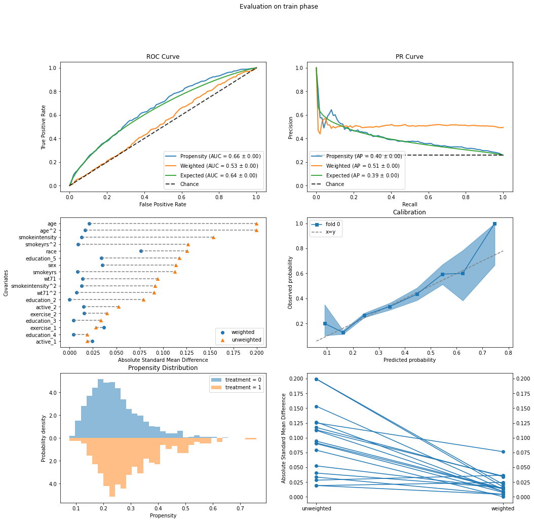
results = evaluate(dr.weight_model, data.X, data.a, data.y)
results.plot_all()
results.evaluated_metrics.prediction_scores

	accuracy	precision	recall	f1	roc_auc	avg_precision	hinge	matthews	0_1	brier	confusion_matrix	roc_curve	pr_curve
0	0.749042	0.613636	0.066998	0.120805	0.660555	0.400766	1.10319	0.138572	0.250958	0.179105	[[1146, 17], [376, 27]]	([0.0, 0.0, 0.0, 0.0008598452278589854, 0.0008...	([0.25767263427109977, 0.2571976967370441, 0.2...

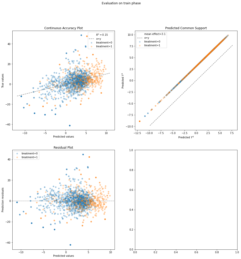
results = evaluate(dr, data.X, data.a, data.y)
results.plot_all()                                        
results.evaluated_metrics

	expvar	mae	mse	mdae	r2
model_strata
actual	0.147487	5.278826	52.901286	4.039940	0.147487
0	0.125392	4.999575	48.489150	3.806782	0.125392
1	0.140264	6.084701	65.634076	4.552075	0.140264